Fitting three machine learning models using the `TidyModel` Framework.

NOTE: Original code for exercise was divided into separate scripts in respective repo.
## OBJECTIVE

Data

Loading Data

Loading all the default settings and preliminary programs.

Path to Processed Data and loading of cleaned data

data_location <- here::here("data","processed_data","processeddata.rds")
data<- readRDS(data_location)

Reminder: Outcome of interest is Body Temp; Categorical outcome is Nausea; Predictor= RunnyNose

glimpse(data)

## Rows: 730
## Columns: 32
## $ SwollenLymphNodes <fct> Yes, Yes, Yes, Yes, Yes, No, No, No, Yes, No, Yes, Y~
## $ ChestCongestion   <fct> No, Yes, Yes, Yes, No, No, No, Yes, Yes, Yes, Yes, Y~
## $ ChillsSweats      <fct> No, No, Yes, Yes, Yes, Yes, Yes, Yes, Yes, No, Yes, ~
## $ NasalCongestion   <fct> No, Yes, Yes, Yes, No, No, No, Yes, Yes, Yes, Yes, Y~
## $ CoughYN           <fct> Yes, Yes, No, Yes, No, Yes, Yes, Yes, Yes, Yes, No, ~
## $ Sneeze            <fct> No, No, Yes, Yes, No, Yes, No, Yes, No, No, No, No, ~
## $ Fatigue           <fct> Yes, Yes, Yes, Yes, Yes, Yes, Yes, Yes, Yes, Yes, Ye~
## $ SubjectiveFever   <fct> Yes, Yes, Yes, Yes, Yes, Yes, Yes, Yes, Yes, No, Yes~
## $ Headache          <fct> Yes, Yes, Yes, Yes, Yes, Yes, No, Yes, Yes, Yes, Yes~
## $ Weakness          <fct> Mild, Severe, Severe, Severe, Moderate, Moderate, Mi~
## $ WeaknessYN        <fct> Yes, Yes, Yes, Yes, Yes, Yes, Yes, Yes, Yes, Yes, Ye~
## $ CoughIntensity    <fct> Severe, Severe, Mild, Moderate, None, Moderate, Seve~
## $ CoughYN2          <fct> Yes, Yes, Yes, Yes, No, Yes, Yes, Yes, Yes, Yes, Yes~
## $ Myalgia           <fct> Mild, Severe, Severe, Severe, Mild, Moderate, Mild, ~
## $ MyalgiaYN         <fct> Yes, Yes, Yes, Yes, Yes, Yes, Yes, Yes, Yes, Yes, Ye~
## $ RunnyNose         <fct> No, No, Yes, Yes, No, No, Yes, Yes, Yes, Yes, No, No~
## $ AbPain            <fct> No, No, Yes, No, No, No, No, No, No, No, Yes, Yes, N~
## $ ChestPain         <fct> No, No, Yes, No, No, Yes, Yes, No, No, No, No, Yes, ~
## $ Diarrhea          <fct> No, No, No, No, No, Yes, No, No, No, No, No, No, No,~
## $ EyePn             <fct> No, No, No, No, Yes, No, No, No, No, No, Yes, No, Ye~
## $ Insomnia          <fct> No, No, Yes, Yes, Yes, No, No, Yes, Yes, Yes, Yes, Y~
## $ ItchyEye          <fct> No, No, No, No, No, No, No, No, No, No, No, No, Yes,~
## $ Nausea            <fct> No, No, Yes, Yes, Yes, Yes, No, No, Yes, Yes, Yes, Y~
## $ EarPn             <fct> No, Yes, No, Yes, No, No, No, No, No, No, No, Yes, Y~
## $ Hearing           <fct> No, Yes, No, No, No, No, No, No, No, No, No, No, No,~
## $ Pharyngitis       <fct> Yes, Yes, Yes, Yes, Yes, Yes, Yes, No, No, No, Yes, ~
## $ Breathless        <fct> No, No, Yes, No, No, Yes, No, No, No, Yes, No, Yes, ~
## $ ToothPn           <fct> No, No, Yes, No, No, No, No, No, Yes, No, No, Yes, N~
## $ Vision            <fct> No, No, No, No, No, No, No, No, No, No, No, No, No, ~
## $ Vomit             <fct> No, No, No, No, No, No, Yes, No, No, No, Yes, Yes, N~
## $ Wheeze            <fct> No, No, No, Yes, No, Yes, No, No, No, No, No, Yes, N~
## $ BodyTemp          <dbl> 98.3, 100.4, 100.8, 98.8, 100.5, 98.4, 102.5, 98.4, ~

Feature / Variable removal

Remove severity score data

OrderedData<-data%>%
  #remove YN variables for those variables with severity factors
  select(-WeaknessYN,-CoughYN,-MyalgiaYN,-CoughYN2)%>%
  #code symptom severity factors as ordinal
  mutate(Weakness=as.ordered(Weakness), CoughIntensity=as.ordered(CoughIntensity), Myalgia=as.ordered(Myalgia))%>%
  #Order severity in ordered factors: None<mild<Moderate<Severee
 mutate_at(vars(Weakness, CoughIntensity, Myalgia),
           list(~factor(.,levels = c("None","Mild","Moderate","Severe"),ordered = TRUE)))

summary(OrderedData)

##  SwollenLymphNodes ChestCongestion ChillsSweats NasalCongestion Sneeze   
##  No :418           No :323         No :130      No :167         No :339  
##  Yes:312           Yes:407         Yes:600      Yes:563         Yes:391  
##                                                                          
##                                                                          
##                                                                          
##                                                                          
##  Fatigue   SubjectiveFever Headache      Weakness    CoughIntensity
##  No : 64   No :230         No :115   None    : 49   None    : 47   
##  Yes:666   Yes:500         Yes:615   Mild    :223   Mild    :154   
##                                      Moderate:338   Moderate:357   
##                                      Severe  :120   Severe  :172   
##                                                                    
##                                                                    
##      Myalgia    RunnyNose AbPain    ChestPain Diarrhea  EyePn     Insomnia 
##  None    : 79   No :211   No :639   No :497   No :631   No :617   No :315  
##  Mild    :213   Yes:519   Yes: 91   Yes:233   Yes: 99   Yes:113   Yes:415  
##  Moderate:325                                                              
##  Severe  :113                                                              
##                                                                            
##                                                                            
##  ItchyEye  Nausea    EarPn     Hearing   Pharyngitis Breathless ToothPn  
##  No :551   No :475   No :568   No :700   No :119     No :436    No :565  
##  Yes:179   Yes:255   Yes:162   Yes: 30   Yes:611     Yes:294    Yes:165  
##                                                                          
##                                                                          
##                                                                          
##                                                                          
##  Vision    Vomit     Wheeze       BodyTemp     
##  No :711   No :652   No :510   Min.   : 97.20  
##  Yes: 19   Yes: 78   Yes:220   1st Qu.: 98.20  
##                                Median : 98.50  
##                                Mean   : 98.94  
##                                3rd Qu.: 99.30  
##                                Max.   :103.10

Low variance predictors view summary of Ordered Data <50 entries

Mod11Data<-OrderedData%>%
  select(-Hearing, -Vision)

glimpse(Mod11Data)

## Rows: 730
## Columns: 26
## $ SwollenLymphNodes <fct> Yes, Yes, Yes, Yes, Yes, No, No, No, Yes, No, Yes, Y~
## $ ChestCongestion   <fct> No, Yes, Yes, Yes, No, No, No, Yes, Yes, Yes, Yes, Y~
## $ ChillsSweats      <fct> No, No, Yes, Yes, Yes, Yes, Yes, Yes, Yes, No, Yes, ~
## $ NasalCongestion   <fct> No, Yes, Yes, Yes, No, No, No, Yes, Yes, Yes, Yes, Y~
## $ Sneeze            <fct> No, No, Yes, Yes, No, Yes, No, Yes, No, No, No, No, ~
## $ Fatigue           <fct> Yes, Yes, Yes, Yes, Yes, Yes, Yes, Yes, Yes, Yes, Ye~
## $ SubjectiveFever   <fct> Yes, Yes, Yes, Yes, Yes, Yes, Yes, Yes, Yes, No, Yes~
## $ Headache          <fct> Yes, Yes, Yes, Yes, Yes, Yes, No, Yes, Yes, Yes, Yes~
## $ Weakness          <ord> Mild, Severe, Severe, Severe, Moderate, Moderate, Mi~
## $ CoughIntensity    <ord> Severe, Severe, Mild, Moderate, None, Moderate, Seve~
## $ Myalgia           <ord> Mild, Severe, Severe, Severe, Mild, Moderate, Mild, ~
## $ RunnyNose         <fct> No, No, Yes, Yes, No, No, Yes, Yes, Yes, Yes, No, No~
## $ AbPain            <fct> No, No, Yes, No, No, No, No, No, No, No, Yes, Yes, N~
## $ ChestPain         <fct> No, No, Yes, No, No, Yes, Yes, No, No, No, No, Yes, ~
## $ Diarrhea          <fct> No, No, No, No, No, Yes, No, No, No, No, No, No, No,~
## $ EyePn             <fct> No, No, No, No, Yes, No, No, No, No, No, Yes, No, Ye~
## $ Insomnia          <fct> No, No, Yes, Yes, Yes, No, No, Yes, Yes, Yes, Yes, Y~
## $ ItchyEye          <fct> No, No, No, No, No, No, No, No, No, No, No, No, Yes,~
## $ Nausea            <fct> No, No, Yes, Yes, Yes, Yes, No, No, Yes, Yes, Yes, Y~
## $ EarPn             <fct> No, Yes, No, Yes, No, No, No, No, No, No, No, Yes, Y~
## $ Pharyngitis       <fct> Yes, Yes, Yes, Yes, Yes, Yes, Yes, No, No, No, Yes, ~
## $ Breathless        <fct> No, No, Yes, No, No, Yes, No, No, No, Yes, No, Yes, ~
## $ ToothPn           <fct> No, No, Yes, No, No, No, No, No, Yes, No, No, Yes, N~
## $ Vomit             <fct> No, No, No, No, No, No, Yes, No, No, No, Yes, Yes, N~
## $ Wheeze            <fct> No, No, No, Yes, No, Yes, No, No, No, No, No, Yes, N~
## $ BodyTemp          <dbl> 98.3, 100.4, 100.8, 98.8, 100.5, 98.4, 102.5, 98.4, ~

location to save file

save_data_location <- here::here("data","processed_data","Mod11Data.rds")

saveRDS(Mod11Data, file = save_data_location)

Summary of data

skim(Mod11Data) # use skimmer to summarize data

Data summary
Name	Mod11Data
Number of rows	730
Number of columns	26
_______________________
Column type frequency:
factor	25
numeric	1
________________________
Group variables	None

Variable type: factor

skim_variable	complete_rate	ordered	n_unique	top_counts
SwollenLymphNodes	1	FALSE	2	No: 418, Yes: 312
ChestCongestion	1	FALSE	2	Yes: 407, No: 323
ChillsSweats	1	FALSE	2	Yes: 600, No: 130
NasalCongestion	1	FALSE	2	Yes: 563, No: 167
Sneeze	1	FALSE	2	Yes: 391, No: 339
Fatigue	1	FALSE	2	Yes: 666, No: 64
SubjectiveFever	1	FALSE	2	Yes: 500, No: 230
Headache	1	FALSE	2	Yes: 615, No: 115
Weakness	1	TRUE	4	Mod: 338, Mil: 223, Sev: 120, Non: 49
CoughIntensity	1	TRUE	4	Mod: 357, Sev: 172, Mil: 154, Non: 47
Myalgia	1	TRUE	4	Mod: 325, Mil: 213, Sev: 113, Non: 79
RunnyNose	1	FALSE	2	Yes: 519, No: 211
AbPain	1	FALSE	2	No: 639, Yes: 91
ChestPain	1	FALSE	2	No: 497, Yes: 233
Diarrhea	1	FALSE	2	No: 631, Yes: 99
EyePn	1	FALSE	2	No: 617, Yes: 113
Insomnia	1	FALSE	2	Yes: 415, No: 315
ItchyEye	1	FALSE	2	No: 551, Yes: 179
Nausea	1	FALSE	2	No: 475, Yes: 255
EarPn	1	FALSE	2	No: 568, Yes: 162
Pharyngitis	1	FALSE	2	Yes: 611, No: 119
Breathless	1	FALSE	2	No: 436, Yes: 294
ToothPn	1	FALSE	2	No: 565, Yes: 165
Vomit	1	FALSE	2	No: 652, Yes: 78
Wheeze	1	FALSE	2	No: 510, Yes: 220

Variable type: numeric

skim_variable	n_missing	complete_rate	mean	sd	p0	p25	p50	p75	p100	hist
BodyTemp	0	1	98.94	1.2	97.2	98.2	98.5	99.3	103.1	▇▇▂▁▁

Set Seed

#set random seed to 123 for reproducibility
set.seed(123)

Training and Testing Split

#split dataset into 70% training, 30% testing
#use BodyTemp as stratification
data_split <- initial_split(Mod11Data, 
                            prop = 7/10,
                            strata = BodyTemp)

#create dataframes for the split data
train_data <- training(data_split)
test_data <- testing(data_split)

5-fold Cross Validation

folds <- 
  vfold_cv(train_data,
           v = 5,
           repeats = 5,
           strata = BodyTemp)

Body Temperature vs. all predictors

Below I am creating the new full model recipe for body temperature against all predictors, We have the recipe program add dummy values for all nominal predictors– BodyTemp

Mod11_rec<-
  recipe(BodyTemp~., train_data)%>%
  step_dummy(all_nominal_predictors())

Null Model Perfomance

A null model is one with out any predictors. In this case, this predicts the mean of the outcome. We will compute the RMSE for this and compare with the final model.

Create Null Model

#create null model
null_mod <- 
  null_model() %>%
  set_engine("parsnip") %>%
  set_mode("regression")

#add recipe and model into workflow
null_wflow <- 
  workflow() %>%
  add_recipe(Mod11_rec) %>%
  add_model(null_mod)

Fitting the null model to training data

null_train <- 
  null_wflow %>%
  fit(data = train_data)

#summary of null model with training data to get mean (which in this case is the RMSE)
tidy(null_train)

## # A tibble: 1 x 1
##   value
##   <dbl>
## 1  98.9

Fitting the null model to test data

null_test <- 
  null_wflow %>%
  fit(data = test_data)

#summary of null model with test data to get mean (which in this case is the RMSE)
tidy(null_train)

## # A tibble: 1 x 1
##   value
##   <dbl>
## 1  98.9

Null RMSE values

#RMSE for training data
null_RMSE_train <- 
  tibble(
    rmse = rmse_vec(
      truth = train_data$BodyTemp,
      estimate = rep(mean(train_data$BodyTemp), 
                     nrow(train_data))),
    SE = 0,
    model = "Null - Train")

null_RMSE_train

## # A tibble: 1 x 3
##    rmse    SE model       
##   <dbl> <dbl> <chr>       
## 1  1.21     0 Null - Train

#RMSE for testing data
null_RMSE_test <- 
  tibble(
    rmse = rmse_vec(
      truth = test_data$BodyTemp,
      estimate = rep(mean(test_data$BodyTemp), 
                     nrow(test_data))),
    SE = 0,
    model = "Null - Test")

null_RMSE_test

## # A tibble: 1 x 3
##    rmse    SE model      
##   <dbl> <dbl> <chr>      
## 1  1.16     0 Null - Test

Decision Tree Model

AKA, Tree Model, it is a non-parametric supervised learning method used for classification and regression. The goal is to create a model that predicts the value of a target variable by learning simple decision rules inferred from the data features. A tree can be seen as a piecewise constant approximation.

Structure of this code is biased from TidyModels Tutorial for Tuning.

Model Evaluation

Defining the tree model.

tree_mod<-
  #parsnip package - tuning hyperparameters-- with set engine and mode
  decision_tree(
    # tune() is a placeholder for parsnip to ID
    cost_complexity = tune(),
    tree_depth = tune(),
    min_n = tune())%>%
  set_engine("rpart")%>%
  set_mode("regression") #use regression instead of classification

tree_mod

## Decision Tree Model Specification (regression)
## 
## Main Arguments:
##   cost_complexity = tune()
##   tree_depth = tune()
##   min_n = tune()
## 
## Computational engine: rpart

Tuning grid specification

tree_grid<-
  # grid_regular- chooses sensible values for each hyper parameter
  grid_regular(
    cost_complexity(),
    tree_depth(),
    min_n(), #add to increase 25x
    levels = 5
  )

tree_grid

## # A tibble: 125 x 3
##    cost_complexity tree_depth min_n
##              <dbl>      <int> <int>
##  1    0.0000000001          1     2
##  2    0.0000000178          1     2
##  3    0.00000316            1     2
##  4    0.000562              1     2
##  5    0.1                   1     2
##  6    0.0000000001          4     2
##  7    0.0000000178          4     2
##  8    0.00000316            4     2
##  9    0.000562              4     2
## 10    0.1                   4     2
## # ... with 115 more rows

# view the tree depth
tree_grid%>%
  count(tree_depth)

## # A tibble: 5 x 2
##   tree_depth     n
##        <int> <int>
## 1          1    25
## 2          4    25
## 3          8    25
## 4         11    25
## 5         15    25

Define workflow

tree_WF<-
  workflow()%>%
  add_model(tree_mod)%>% # Preprocessor, decision tree and added dummy
  add_recipe(Mod11_rec) # Model- recipe from `Recipe 1` chunk, features BodyTemp and all other predictors

tree_WF

## == Workflow ====================================================================
## Preprocessor: Recipe
## Model: decision_tree()
## 
## -- Preprocessor ----------------------------------------------------------------
## 1 Recipe Step
## 
## * step_dummy()
## 
## -- Model -----------------------------------------------------------------------
## Decision Tree Model Specification (regression)
## 
## Main Arguments:
##   cost_complexity = tune()
##   tree_depth = tune()
##   min_n = tune()
## 
## Computational engine: rpart

Cross-Validation and tune_grid() for additional tuning

#tune the model with previously specified CV and RMSE
tree_res <- 
  tree_WF %>%
  tune_grid(
    resamples=folds,
    grid= tree_grid,
    metric_set(rmse))

## ! Fold1, Repeat1: internal: A correlation computation is required, but `estimate` is const...

## ! Fold2, Repeat1: internal: A correlation computation is required, but `estimate` is const...

## ! Fold3, Repeat1: internal: A correlation computation is required, but `estimate` is const...

## ! Fold4, Repeat1: internal: A correlation computation is required, but `estimate` is const...

## ! Fold5, Repeat1: internal: A correlation computation is required, but `estimate` is const...

## ! Fold1, Repeat2: internal: A correlation computation is required, but `estimate` is const...

## ! Fold2, Repeat2: internal: A correlation computation is required, but `estimate` is const...

## ! Fold3, Repeat2: internal: A correlation computation is required, but `estimate` is const...

## ! Fold4, Repeat2: internal: A correlation computation is required, but `estimate` is const...

## ! Fold5, Repeat2: internal: A correlation computation is required, but `estimate` is const...

## ! Fold1, Repeat3: internal: A correlation computation is required, but `estimate` is const...

## ! Fold2, Repeat3: internal: A correlation computation is required, but `estimate` is const...

## ! Fold3, Repeat3: internal: A correlation computation is required, but `estimate` is const...

## ! Fold4, Repeat3: internal: A correlation computation is required, but `estimate` is const...

## ! Fold5, Repeat3: internal: A correlation computation is required, but `estimate` is const...

## ! Fold1, Repeat4: internal: A correlation computation is required, but `estimate` is const...

## ! Fold2, Repeat4: internal: A correlation computation is required, but `estimate` is const...

## ! Fold3, Repeat4: internal: A correlation computation is required, but `estimate` is const...

## ! Fold4, Repeat4: internal: A correlation computation is required, but `estimate` is const...

## ! Fold5, Repeat4: internal: A correlation computation is required, but `estimate` is const...

## ! Fold1, Repeat5: internal: A correlation computation is required, but `estimate` is const...

## ! Fold2, Repeat5: internal: A correlation computation is required, but `estimate` is const...

## ! Fold3, Repeat5: internal: A correlation computation is required, but `estimate` is const...

## ! Fold4, Repeat5: internal: A correlation computation is required, but `estimate` is const...

## ! Fold5, Repeat5: internal: A correlation computation is required, but `estimate` is const...

Decision Tree Metrics and Plotting - Model Evaluation

autoplot

creates a defaulted visualization

tree_res%>%
  autoplot()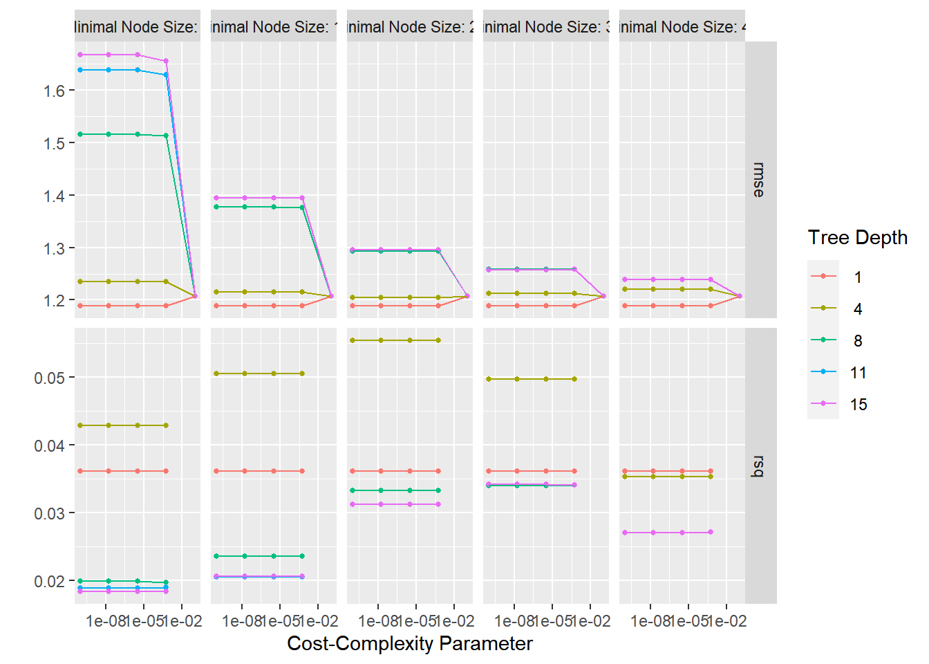

Finding the Best Tree Model

best_tree <- 
  tree_res %>%
  select_best("rmse") #function to pull out the single set of hyperparameter values for best decision tree model

best_tree

## # A tibble: 1 x 4
##   cost_complexity tree_depth min_n .config               
##             <dbl>      <int> <int> <chr>                 
## 1    0.0000000001          1     2 Preprocessor1_Model001

# results for tree depth and cost complexity that max the accuracy in the dataset of cell images.

Finalize Decision Tree

Final Workflow

final_WF <- 
  tree_WF %>% 
  finalize_workflow(best_tree) # already pulled best "RMSE" tree

final_WF

## == Workflow ====================================================================
## Preprocessor: Recipe
## Model: decision_tree()
## 
## -- Preprocessor ----------------------------------------------------------------
## 1 Recipe Step
## 
## * step_dummy()
## 
## -- Model -----------------------------------------------------------------------
## Decision Tree Model Specification (regression)
## 
## Main Arguments:
##   cost_complexity = 1e-10
##   tree_depth = 1
##   min_n = 2
## 
## Computational engine: rpart

Last Fit

Fitting with fit()

final_fit<-
  final_WF%>%
  fit(train_data)

Predicting outcomes for final model (training data)

tree_pred<- 
  predict(final_fit,
          train_data) #testing fit with the training split

Plotting final tree

rpart.plot(extract_fit_parsnip(final_fit)$fit)

## Warning: Cannot retrieve the data used to build the model (model.frame: object '..y' not found).
## To silence this warning:
##     Call rpart.plot with roundint=FALSE,
##     or rebuild the rpart model with model=TRUE.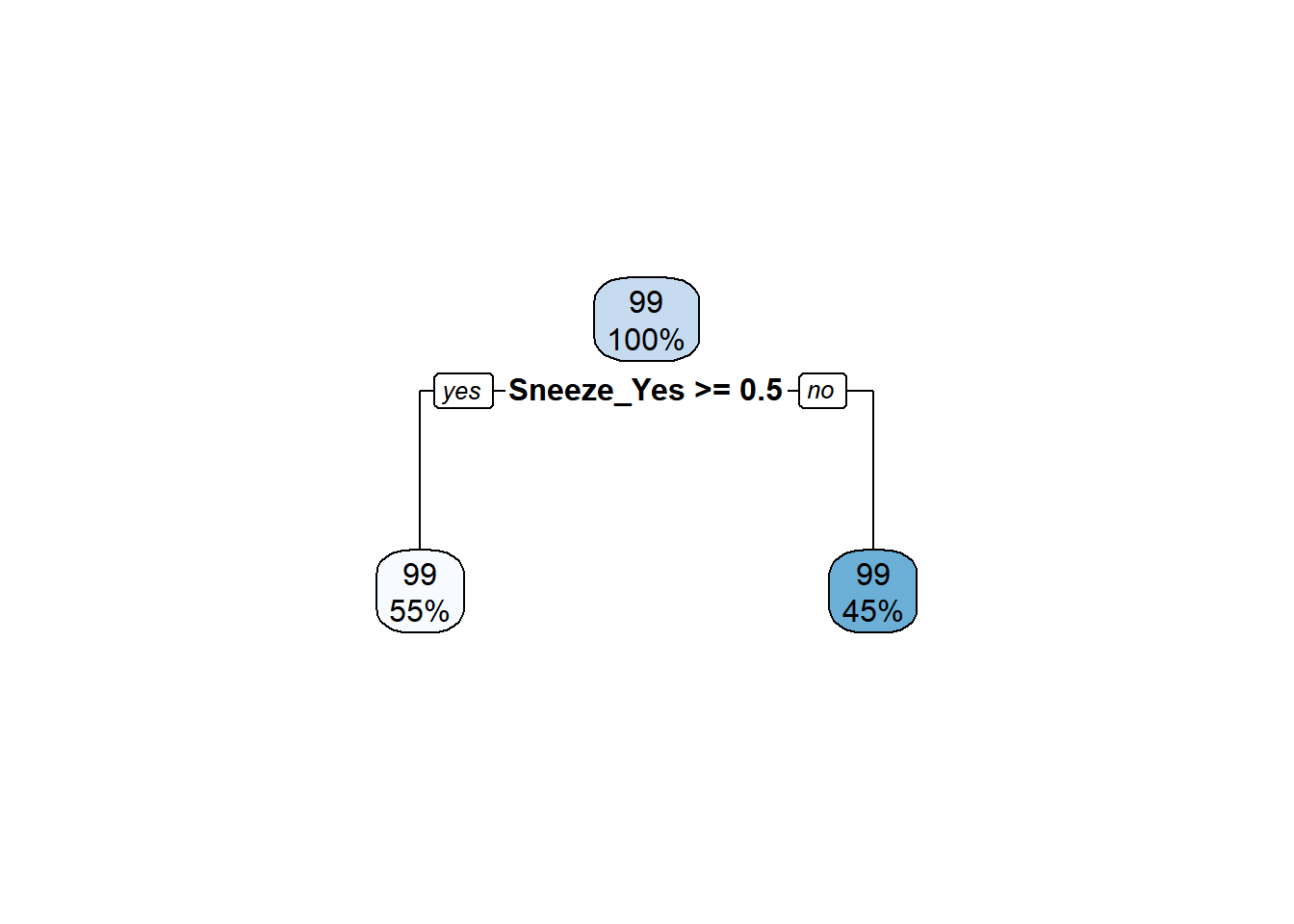

Plotting

Predictions and Interval Fit

#predicted versus observed
plot(tree_pred$.pred,train_data$BodyTemp)
abline(a=0,b=1, col = 'red') #45 degree line, along which the results should fall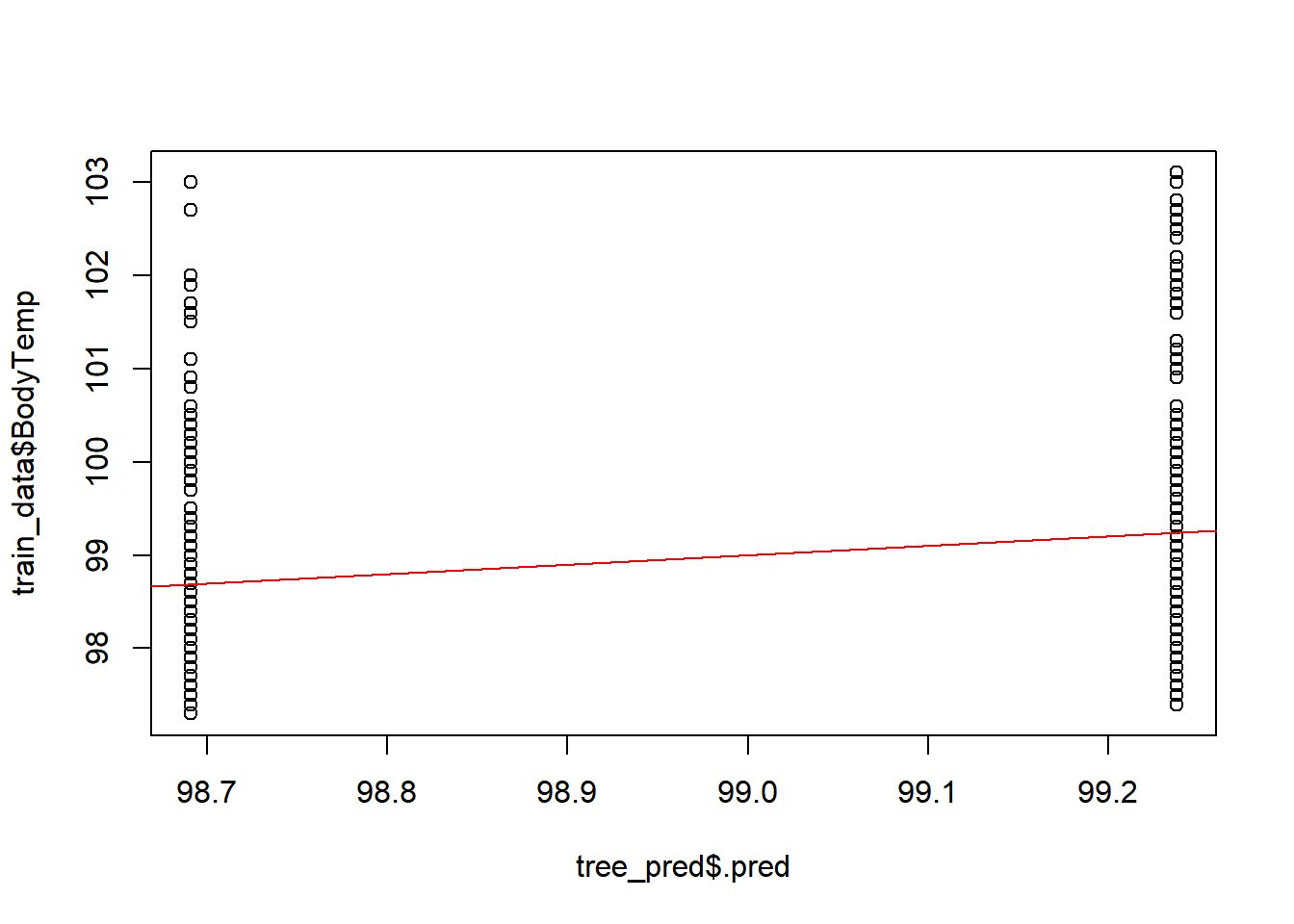

### Residuals

plot(tree_pred$.pred-train_data$BodyTemp)
abline(a=0,b=0, col = 'red') #straight line, along which the results should fall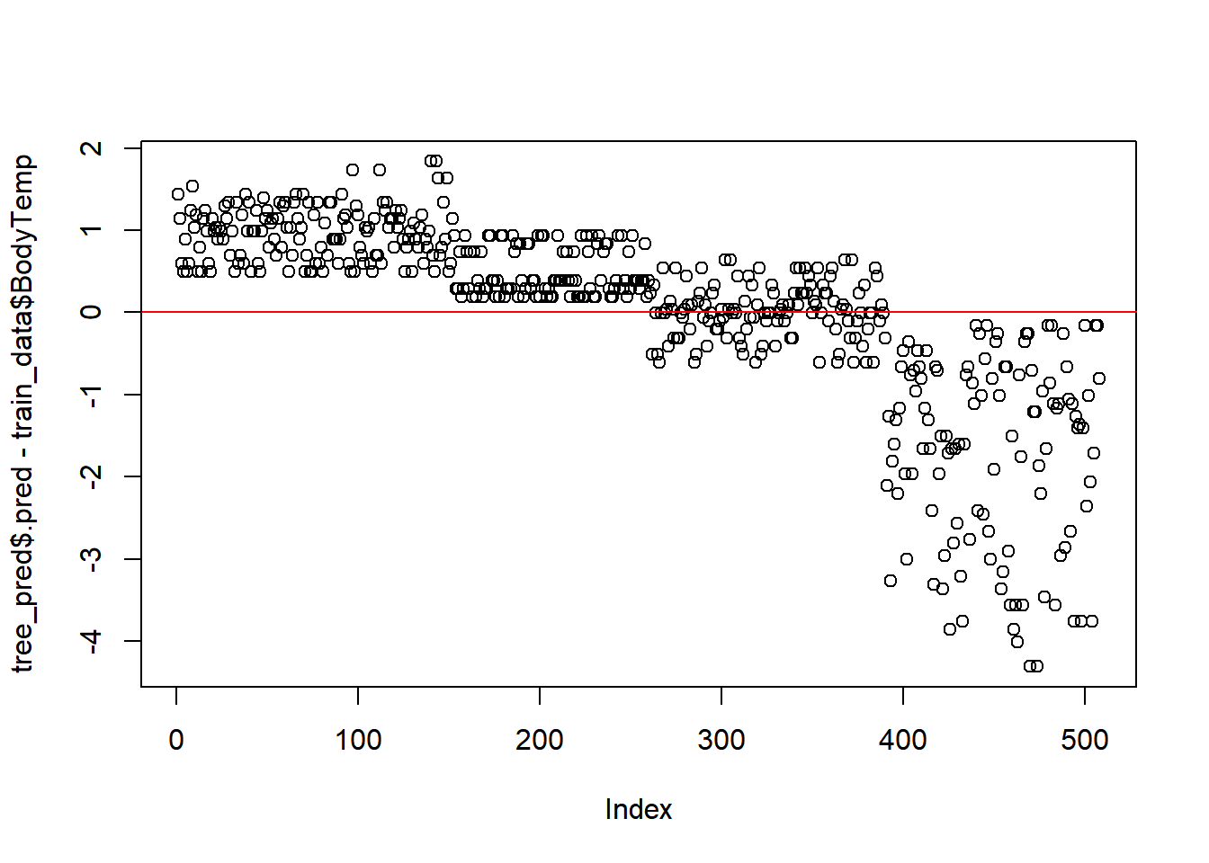

Tree Performance

tree_perfomance <- tree_res %>% show_best(n = 5)

## Warning: No value of `metric` was given; metric 'rmse' will be used.

print(tree_perfomance)

## # A tibble: 5 x 9
##   cost_complexity tree_depth min_n .metric .estimator  mean     n std_err
##             <dbl>      <int> <int> <chr>   <chr>      <dbl> <int>   <dbl>
## 1    0.0000000001          1     2 rmse    standard    1.19    25  0.0181
## 2    0.0000000178          1     2 rmse    standard    1.19    25  0.0181
## 3    0.00000316            1     2 rmse    standard    1.19    25  0.0181
## 4    0.000562              1     2 rmse    standard    1.19    25  0.0181
## 5    0.0000000001          1    11 rmse    standard    1.19    25  0.0181
## # ... with 1 more variable: .config <chr>

Compare model performance to null model

tree_RMSE<-
  tree_res%>% #CV and tuned grid recipe
  show_best(n=1)%>%
  transmute( # row names in the performance output
    rmse=round(mean,2),
    SE=round(std_err,2),
    model="Tree")

## Warning: No value of `metric` was given; metric 'rmse' will be used.

tree_RMSE

## # A tibble: 1 x 3
##    rmse    SE model
##   <dbl> <dbl> <chr>
## 1  1.19  0.02 Tree

Comments:

The best performing tree model predicts two values.

LASSO for Linear Regression

Type of linear regression that uses shrinkage (data values shrunk towards a central point, mean).

NOTE: Aspects from the Decision Tree Model will be used to perform a LASSO Linear Regression. Code for this section may be taken from (TidyModels Tutorial Case Study)[https://www.tidymodels.org/start/case-study/].

LASSO Setup

Building/define the LASSO model

lasso_model <- linear_reg() %>%
  set_mode("regression") %>%           
  set_engine("glmnet") %>% #glmnet engine to specify a penelized logistic regression model
  set_args(penalty = tune(), 
           mixture = 1) #mixture 1 => means we use the LASSO model

LASSO WorkFlow

lasso_WF<-
  workflow()%>%
  add_model(lasso_model)%>%
  add_recipe(Mod11_rec)

LASSO Tuning

#specifics for tuning grid = add penalties
lasso_grid <- 
  tibble(penalty = 10^seq(-3, 0, length.out = 30))

#tune model
lasso_tune_rec <- 
  lasso_WF %>% 
  tune_grid(resamples = folds, #tune with CV value pre designated
            grid = lasso_grid,
            control = control_grid(
              save_pred = TRUE
              ),
            metrics = metric_set(rmse) #RMSE as target metric
            )

lasso_tune_rec%>%
  autoplot()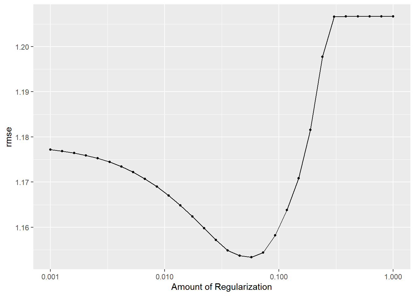

#View top 15 models with lowest RMSEs
lasso_top_models<-
  lasso_tune_rec%>%
  show_best("rmse", n=15)%>%
  arrange(penalty)

lasso_top_models

## # A tibble: 15 x 7
##    penalty .metric .estimator  mean     n std_err .config              
##      <dbl> <chr>   <chr>      <dbl> <int>   <dbl> <chr>                
##  1 0.00530 rmse    standard    1.17    25  0.0167 Preprocessor1_Model08
##  2 0.00672 rmse    standard    1.17    25  0.0167 Preprocessor1_Model09
##  3 0.00853 rmse    standard    1.17    25  0.0167 Preprocessor1_Model10
##  4 0.0108  rmse    standard    1.17    25  0.0167 Preprocessor1_Model11
##  5 0.0137  rmse    standard    1.16    25  0.0167 Preprocessor1_Model12
##  6 0.0174  rmse    standard    1.16    25  0.0167 Preprocessor1_Model13
##  7 0.0221  rmse    standard    1.16    25  0.0168 Preprocessor1_Model14
##  8 0.0281  rmse    standard    1.16    25  0.0169 Preprocessor1_Model15
##  9 0.0356  rmse    standard    1.15    25  0.0169 Preprocessor1_Model16
## 10 0.0452  rmse    standard    1.15    25  0.0169 Preprocessor1_Model17
## 11 0.0574  rmse    standard    1.15    25  0.0169 Preprocessor1_Model18
## 12 0.0728  rmse    standard    1.15    25  0.0170 Preprocessor1_Model19
## 13 0.0924  rmse    standard    1.16    25  0.0172 Preprocessor1_Model20
## 14 0.117   rmse    standard    1.16    25  0.0175 Preprocessor1_Model21
## 15 0.149   rmse    standard    1.17    25  0.0178 Preprocessor1_Model22

#Best tuned LASSO model
lasso_best<-
  lasso_tune_rec%>%
  select_best(metric="rmse")

# finalize workflow with best model
lasso_best_WF <- 
  lasso_WF %>% 
  finalize_workflow(lasso_best)
# fitting best performing model
lasso_best_fit <- 
  lasso_best_WF %>% 
  fit(data = train_data)

lasso_pred <- 
  predict(lasso_best_fit, train_data)

LASSO Evaluation

Tuning parameters plot in LASSO

# extract models from the final fit
x<-
  lasso_best_fit$fit$fit$fit

# plotting the number of predictors and thier changes with the tuning parameter
plot(x, "lambda")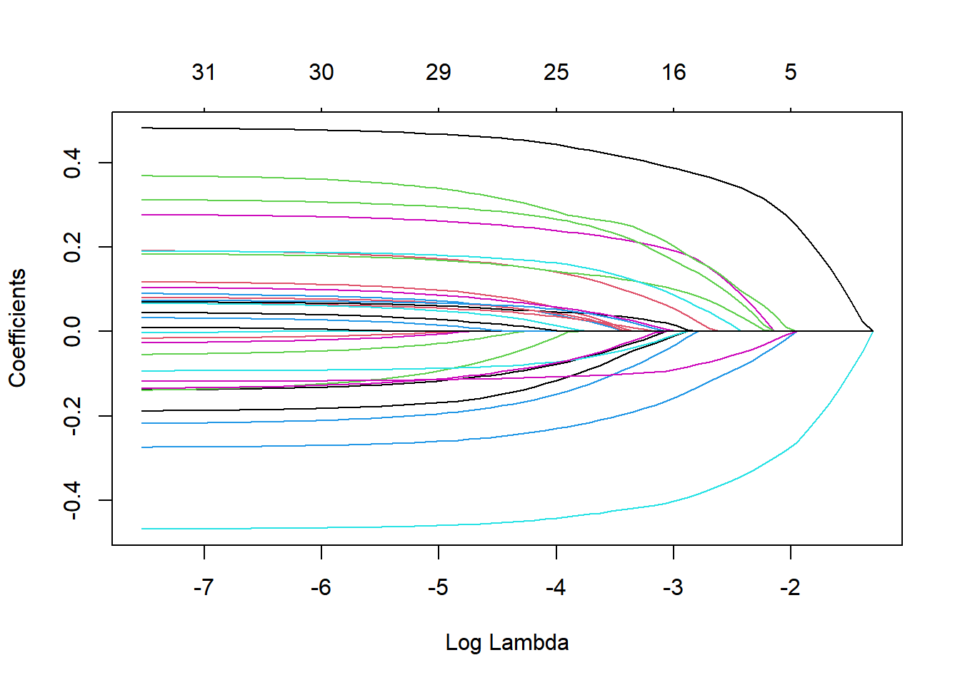

lasso_best_fit%>%
  extract_fit_parsnip()%>%
  tidy()%>%
  filter(estimate!="0") #several estimates are at 0, ignore.

## # A tibble: 13 x 3
##    term                estimate penalty
##    <chr>                  <dbl>   <dbl>
##  1 (Intercept)         98.7      0.0574
##  2 ChestCongestion_Yes  0.0332   0.0574
##  3 ChillsSweats_Yes     0.0894   0.0574
##  4 NasalCongestion_Yes -0.140    0.0574
##  5 Sneeze_Yes          -0.391    0.0574
##  6 Fatigue_Yes          0.178    0.0574
##  7 SubjectiveFever_Yes  0.377    0.0574
##  8 Weakness_1           0.178    0.0574
##  9 Myalgia_2           -0.00994  0.0574
## 10 Myalgia_3            0.0679   0.0574
## 11 RunnyNose_Yes       -0.0825   0.0574
## 12 Nausea_Yes           0.00349  0.0574
## 13 Pharyngitis_Yes      0.148    0.0574

#predicted versus observed from tuned model
plot(lasso_pred$.pred,train_data$BodyTemp, 
     xlim =c(97,104), 
     ylim=c(97,104))
abline(a=0,b=1, col = 'red') #45 degree line, along which the results should fall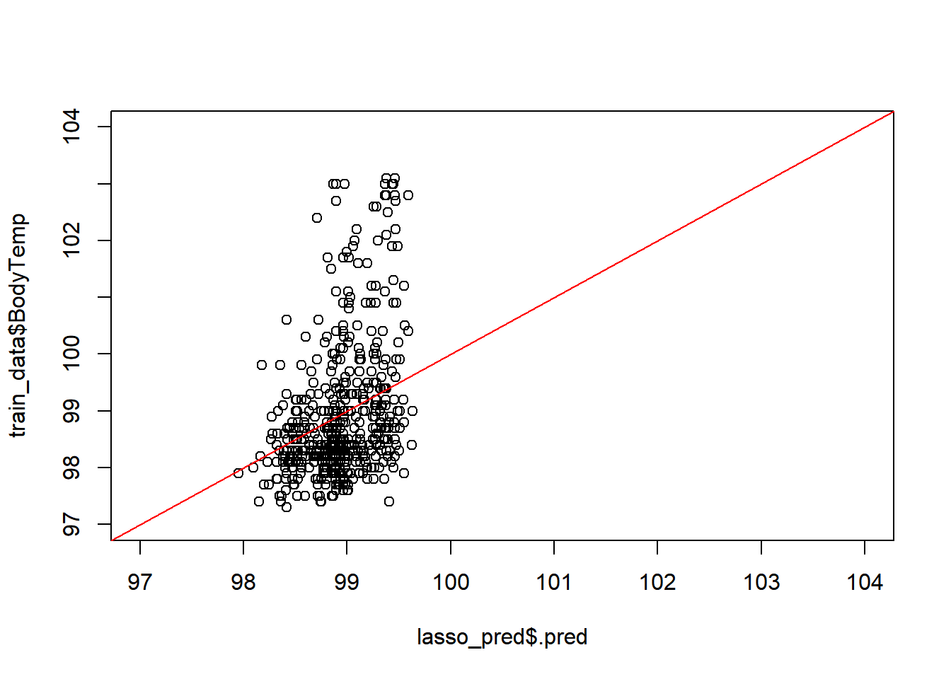

#residuals
plot(lasso_pred$.pred-train_data$BodyTemp)
abline(a=0,b=0, col = 'red')

Ideally, good results should fall along the red line.

#LASSO  Model Performance
lasso_perfomance <- 
  lasso_tune_rec %>% 
  show_best(n = 1)%>%
  print()

## # A tibble: 1 x 7
##   penalty .metric .estimator  mean     n std_err .config              
##     <dbl> <chr>   <chr>      <dbl> <int>   <dbl> <chr>                
## 1  0.0574 rmse    standard    1.15    25  0.0169 Preprocessor1_Model18

#View RMSE comparison with nulls
lasso_RMSE<-
  lasso_tune_rec%>%
  show_best(n=1)%>%
  transmute(
    rmse= round(mean,2),
    SE= round(std_err,2),
    model="LASSO"
  )

LASSO RMSE mean is lower, just a little, from null train and test values.

Random Forest (RF)

NOTE: Aspects from the Decision Tree Model and LASSO Linear Regressionwill be used to create a Random Forest Model. Code for this section may be taken from TidyModels Tutorial Case Study.

RF Setup

RF_model <- 
  rand_forest() %>%
  set_args(mtry = tune(),     
    trees = tune(),
    min_n = tune()
  ) %>%
  # select the engine/package that underlies the model
  set_engine("ranger",
             num.threads = 18, 
             #for some reason for RF, we need to set this in the engine too
             importance = "permutation") %>%
  # choose either the continuous regression or binary classification mode
  set_mode("regression")

#view identified parameters to be tuned
RF_model%>%
  parameters()

## Collection of 3 parameters for tuning
## 
##  identifier  type    object
##        mtry  mtry nparam[?]
##       trees trees nparam[+]
##       min_n min_n nparam[+]
## 
## Model parameters needing finalization:
##    # Randomly Selected Predictors ('mtry')
## 
## See `?dials::finalize` or `?dials::update.parameters` for more information.

RF WorkFlow

# regression workflow
RF_WF <- 
  workflow() %>%
  add_model(RF_model) %>% 
  add_recipe(Mod11_rec)

print(RF_WF)

## == Workflow ====================================================================
## Preprocessor: Recipe
## Model: rand_forest()
## 
## -- Preprocessor ----------------------------------------------------------------
## 1 Recipe Step
## 
## * step_dummy()
## 
## -- Model -----------------------------------------------------------------------
## Random Forest Model Specification (regression)
## 
## Main Arguments:
##   mtry = tune()
##   trees = tune()
##   min_n = tune()
## 
## Engine-Specific Arguments:
##   num.threads = 18
##   importance = permutation
## 
## Computational engine: ranger

RF Tuning

#tuning grid
RF_grid<-
  expand.grid(mtry = c(3, 4, 5, 6),
              min_n = c(40, 50, 60),
              trees = c(500,1000))

RF_tune_rec<-
  RF_WF%>%
  tune_grid(resamples = folds, #tune with CV value pre designated
            grid = RF_grid, #just created grid of values
            control = control_grid(
              save_pred = TRUE
              ),
            metrics = metric_set(rmse) #RMSE as target metric
            )

RF Evaluation

Autoplot

RF_tune_rec%>%
  autoplot()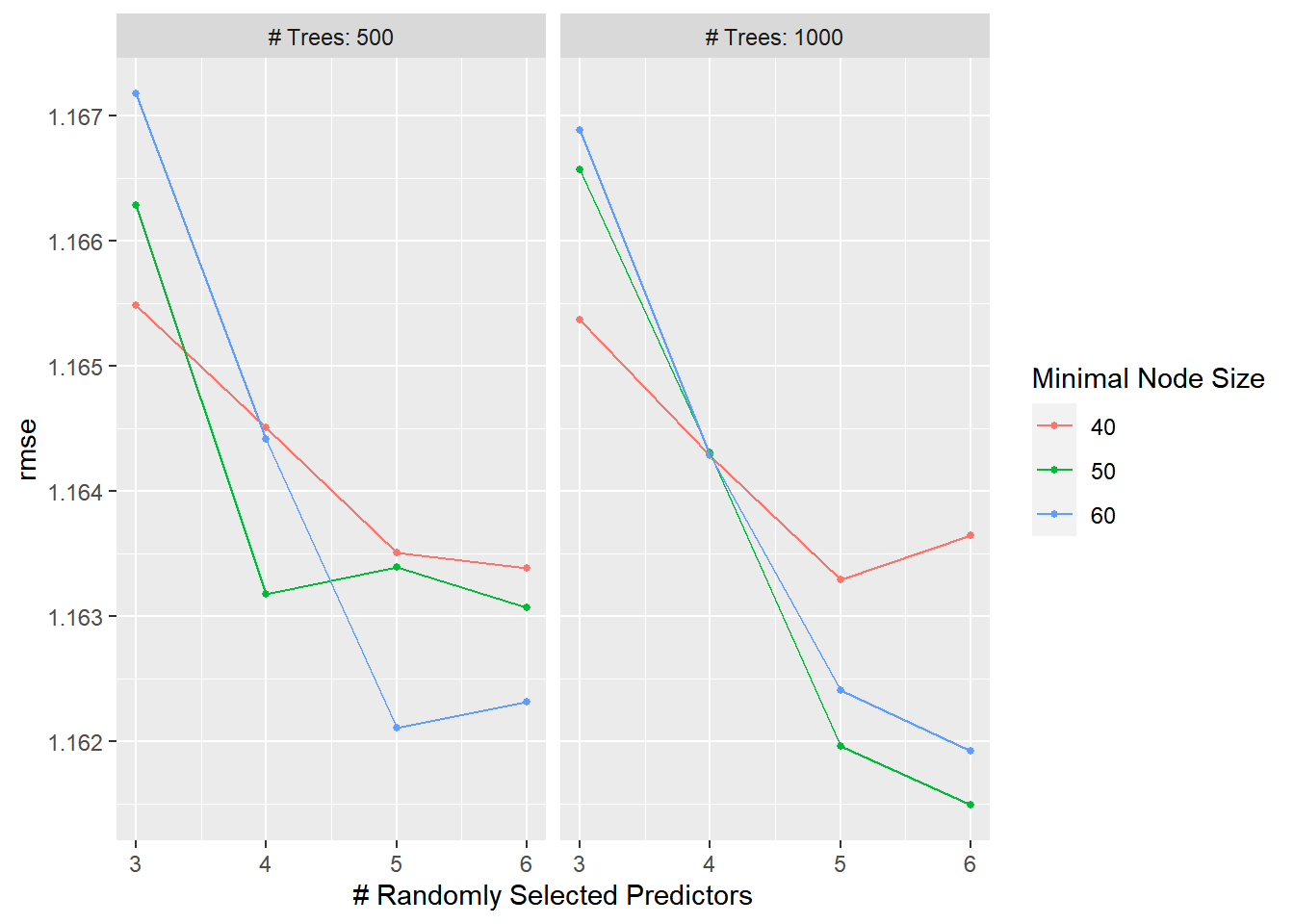

# get the tuned model that performs best 
RF_best <- 
  RF_tune_rec %>%  
  select_best(metric = "rmse")
# finalize workflow with best model
RF_best_WF <- 
  RF_WF %>% 
  finalize_workflow(RF_best)
# fitting best performing model
RF_best_fit <- 
  RF_best_WF %>% 
  fit(data = train_data)
RF_pred <- 
  predict(RF_best_fit, 
          train_data)

Unfortunately, there’s not an easy way to look at a random forest model. Below are examples at looking at the data.
View importance predictors by using vip.

#pull out the fit object
RF_x <- RF_best_fit$fit$fit$fit
#plot variable importance
vip(RF_x, num_features = 20) #can specify features, default is 10.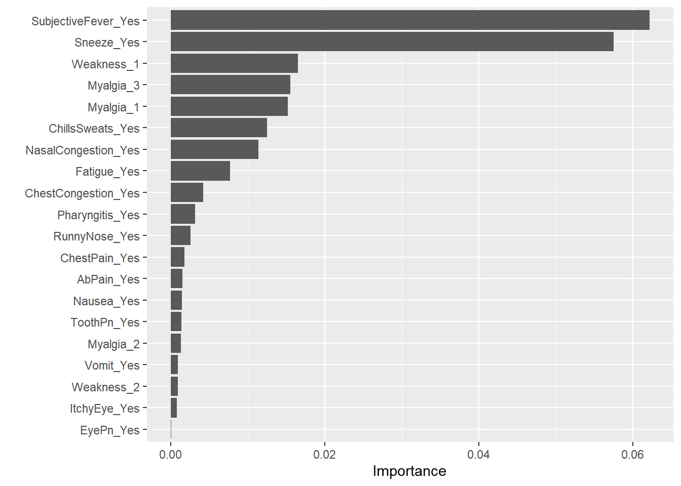

This makes perfect sense that a fever would indicate a difference in BodyTemp– Body Temperature
Plots:

Predicted vs Observed

plot(RF_pred$.pred,
     train_data$BodyTemp, 
     xlim =c(97,103), #x= Actual Body Temp,
     ylim=c(97,103)) # y= predicted body temp
abline(a=0,b=1, col = 'red')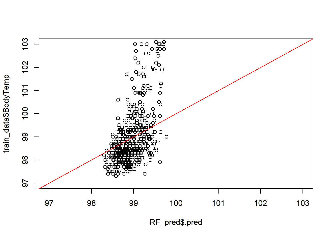

#45 degree line, along which the results should fall

Model fit vs Residuals

#residuals
plot(RF_pred$.pred-train_data$BodyTemp) # Index= Observation Number
#straight line, along which the results should fall
abline(a=0,b=0, col = 'red')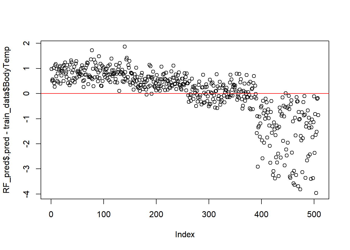

Model Performance

RF_perfomance <- 
  RF_tune_rec %>% 
  show_best(n = 1)

print(RF_perfomance)

## # A tibble: 1 x 9
##    mtry trees min_n .metric .estimator  mean     n std_err .config              
##   <dbl> <dbl> <dbl> <chr>   <chr>      <dbl> <int>   <dbl> <chr>                
## 1     6  1000    50 rmse    standard    1.16    25  0.0168 Preprocessor1_Model20

#View RMSE comparison with nulls
RF_RMSE<-
  RF_tune_rec%>%
  show_best(n=1)%>%
  transmute(
    rmse= round(mean,2),
    SE= round(std_err,2),
    model="RF"
  )

Compared with the nulls this is really no better than the null rmse

Final Model Selection and Evaluation

Compare all RMSE(s) from the models to the Nulls

CompareRMSE<-
  bind_rows(tree_RMSE)%>%
  bind_rows(lasso_RMSE)%>%
  bind_rows(RF_RMSE)%>%
  bind_rows(null_RMSE_train)%>%
  mutate(rmse=round(rmse,2))%>%
  arrange(rmse)%>% #arrange RMSE that is the smallest
  print()

## # A tibble: 4 x 3
##    rmse    SE model       
##   <dbl> <dbl> <chr>       
## 1  1.15  0.02 LASSO       
## 2  1.16  0.02 RF          
## 3  1.19  0.02 Tree        
## 4  1.21  0    Null - Train

None of the models fit the data well. This suggests that the predictor variables in the data set may not be useful in predicting the body temperature of a suspect flu case (outcome).

LASSO model is the best model based on RMSE value being the lowest.

As such, the Lasso model will be evaluated by fitting the LASSO model to the training_data set and evaluate on the test_data.

Performance Check

Fit_Test<-
  lasso_best_WF%>% # wf of the best fit from the training data
  last_fit(split=data_split)

Compare test against training

final_fit <- 
  lasso_best_WF%>% 
  last_fit(data_split)

Final_performance<- 
  final_fit%>% 
  collect_metrics()%>%
  print()

## # A tibble: 2 x 4
##   .metric .estimator .estimate .config             
##   <chr>   <chr>          <dbl> <chr>               
## 1 rmse    standard      1.15   Preprocessor1_Model1
## 2 rsq     standard      0.0291 Preprocessor1_Model1

test_predictions <- 
  final_fit %>% 
  collect_predictions()

Predicted vs Observed

plot(test_predictions$.pred,
     test_data$BodyTemp, #changeed to test data, previously used training 
     xlim =c(97,103), #x= Actual Body Temp,
     ylim=c(97,103)) # y= predicted body temp
abline(a=0,b=1, col = 'red')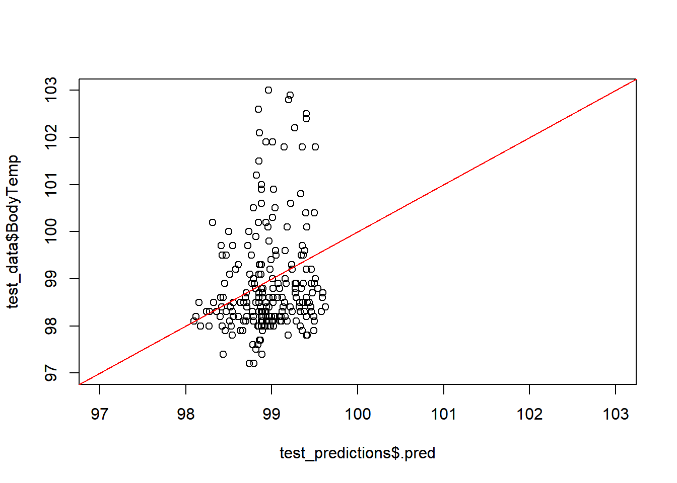

#45 degree line, along which the results should fall

Model fit vs Residuals

#residuals
plot(test_predictions$.pred-test_data$BodyTemp) # Index= Observation Number
#straight line, along which the results should fall
abline(a=0,b=0, col = 'red')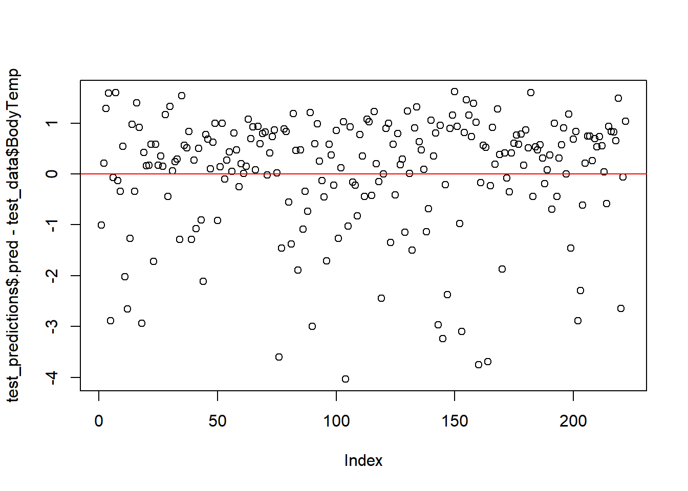

# Comments

LASSO was the best selection from the model types used in this assessment. But it still isn’t great. This suggests that the predictors are not great at predicting the outcome. From the importance predictors the most related to body temp is fever, which makes sense, but in terms of predicting flu– it still has some uncertainty. As there are people who may be positive for flu but may not have severe enough symptoms to warrant getting treated and thus by passing the collection of symptoms.

Machine Learning Results (Mod11)

Fitting three machine learning models using the TidyModel Framework.

Data

Loading Data

Set Seed

Training and Testing Split

5-fold Cross Validation

Body Temperature vs. all predictors

Null Model Perfomance

Create Null Model

Fitting the null model to training data

Fitting the null model to test data

Null RMSE values

Decision Tree Model

Model Evaluation

Defining the tree model.

Tuning grid specification

Define workflow

Cross-Validation and tune_grid() for additional tuning

Decision Tree Metrics and Plotting - Model Evaluation

autoplot

Finding the Best Tree Model

Finalize Decision Tree

Final Workflow

Last Fit

Plotting

Predictions and Interval Fit

Tree Performance

LASSO for Linear Regression

LASSO Setup

LASSO WorkFlow

LASSO Tuning

LASSO Evaluation

Random Forest (RF)

RF Setup

RF WorkFlow

RF Tuning

RF Evaluation

Final Model Selection and Evaluation

Compare all RMSE(s) from the models to the Nulls

Performance Check

Fitting three machine learning models using the `TidyModel` Framework.